Understanding Neural Networks

Let's understand neural networks, both in theory and practically. We'll first discuss the theory behind how a neural network works, while also defining some of the confusing jargon that you may hear around this topic. Then we'll build a basic neural network library from scratch with only numpy (because without it, we'd spend most of our time trying to implement ndarrays). This resource is generally for people who already have seen neural networks to some extent but want to explore them at a deeper level. However, if you are interested and have a good mathematical background, you will likely be able to follow along.

Preliminaries

You should be familiar with differential multivariable calculus and linear algebra, especially vector and matrix operations. For a quick refresher on these concepts, you can check out Paul's Online Notes and his lesson on matrices and vectors.

Proficiency with programming is also important for the practical implementations and background. The implementations are done in Python, but experience with other programming languages is fine.

Review of Vectors and Matrices

We can start by reviewing the basic operations of vectors and matrices. You should already be familair with these operations, but they are here as a reference if you need it as we will be rewriting a lot of expressions later on.

Let $\mathbf{x}, \mathbf{y} \in \mathbb{R}^m$ and $\mathbf{X}, \mathbf{Y} \in \mathbb{R}^{m \times n}$ . The dot product (scalar product) of two vectors is defined as:

\mathbf{x} \cdot \mathbf{y} = \sum_{i = 1}^nx_iy_i = \mathbf{x}^\top\mathbf{y}

The $L_p$ norm of a vector is defined as:

||\mathbf{x}||_p = \left(\sum_{i = 1}^n |x_i|^p\right)^{\frac{1}{p}}

The hadamard (element-wise) product of two matrices is defined as:

\mathbf{X} = \begin{bmatrix}a_{1,1} & \cdots & a_{1,n}\\\vdots & \ddots & \vdots \\ a_{m,1} & \cdots & a_{m,n}\end{bmatrix}

\mathbf{Y} = \begin{bmatrix}b_{1,1} & \cdots & b_{1,n}\\\vdots & \ddots & \vdots \\ b_{m,1} & \cdots & b_{m,n}\end{bmatrix}

\mathbf{X} \odot \mathbf{Y} = \begin{bmatrix}a_{1,1}b_{1,1} & \cdots & a_{1,n}b_{1,n}\\\vdots & \ddots & \vdots \\ a_{m,1}b_{m,1} & \cdots & a_{m,n}b_{m,n}\end{bmatrix}

The matrix-matrix product of two matrices is defined such that, for $\mathbf{A} \in \mathbb{R}^{m \times n}$ and $\mathbf{A} \in \mathbb{R}^{n \times p}$ , $\mathbf{C} = \mathbf{A}\mathbf{B}$ is a $m \times p$ matrix such that:

c_{i,j} = \sum_{k=1}^m a_{i,k}b_{k,j}

Similarly, a matrix-vector product is the dot product of the vector and each column vector of the matrix. In other words,

\mathbf{A}\mathbf{x} = \begin{pmatrix}a_{1,1}x_1 + \cdots + a_{1,n}x_n\\ \vdots \\ a_{m,1}x_1 + \cdots + a_{m,n}x_n\end{pmatrix}

Note that matrix multiplication does not commute.

Some less conventional notation that is often used in machine learning is the addition of a matrices and vectors, where the objects are filled to allow for element-wise operations. For example, in $C = A + b$ , $C_{i,j} = A_{i,j} + b_i$ . This concept is sometimes called broadcasting. This is crucial for understanding the implementation section at the end, so check out numpy's documentation for a more detailed explanation.

Review of Differential Calculus for Neural Networks

Remember that the gradient vector of $f$ at some point $\mathbf{x}$ is going to point in the direction of the greatest increase, and the magnitude is the rate that it is increasing in that direction.

This is an important detail that will become very relevant to neural networks later on.

Assume that the output of our learning model is given by a function $\hat{y} : \mathbb{R}^n \rightarrow \mathbb{R}$ :

\hat{y}(\mathbf{x}, \mathbf{w}) = \sum_{i = 1}^n{x_iw_i} = \mathbf{x} \cdot \mathbf{w}

We also have another function $\mathcal{L} : \mathbb{R}^2 \rightarrow \mathbb{R}$ that is defined as:

\mathcal{L}(y, \hat{y}) = \frac{1}{2}(y - \hat{y})^2

Note that $\hat{y}$ refers to the output function defined above. We now want to compute $\frac{\partial \mathcal{L}}{\partial \mathbf{w}}$ . We will later find that such a situation (with a bit more complexity) will come up very often.

To perform this computation, we need to use the chain rule of multiple variables. Formally written, if $\mathbf{x} = \mathbf{g}(\mathbf{t})$ , and $z = f(\mathbf{x})$ ,

\frac{\partial z}{\partial \mathbf{t}} = {\frac{\partial z}{\partial \mathbf{x}}\frac{\partial \mathbf{x}}{\partial \mathbf{t}}}

For proofs of these rules, see the wikipedia page. To apply the rule to our case, the value of $z$ above is analogous to $\mathcal{L}$ . So,

\frac{\partial \mathcal{L}}{\partial \hat{y}} = -(y - \hat{y}) = \hat{y} - y \\ \frac{\partial \hat{y}}{\partial \mathbf{w}} = \mathbf{x}

\frac{\partial \mathcal{L}}{\partial \mathbf{w}} = {\frac{\partial \mathcal{L}}{\partial \hat{y}}\frac{\partial \hat{y}}{\partial \mathbf{w}}} = \mathbf{x}(\hat{y} - y)

This computation that we've just done will prove useful in the future, as you'll find out soon.

Linear Regression

Neural networks, modeled broadly around the concept of a human brain, can be thought of as really good function approximators.

They are often considered "black box" algorithms because, although they can approximate functions with relatively high accuracy, it can be challenging to draw patterns and relationships between data by studying the outputs and parameters of the algorithm. This will become more apparent as you begin to understand how these black boxes work.

Machine learning models generally need to be trained, or fit, to some data. The data used to train the model is called the training data, and the data used to test the model is called the testing data.

We can stay away from the concept of a "neural network" for a bit and look at something that might be more familiar: linear regression.

Say we have a matrix of data $\mathcal{X}$ , where each column vector $\mathbf{x}$ represents a single data sample.

Generally, the data samples are indexed using $i$ , where $\mathbf{x}^{(i)}$ represents the $i$ th sample and $y^{(i)}$ represents the respective label. The equation for linear regression is given by the general equation of a linear line. Note that we generally use $\hat{y}$ to represent the predicted value.

\hat{y} = w_1x_1 + w_2x_2 + \cdots + w_nx_n + b = \mathbf{w}^\top \mathbf{x} + b

The $b$ value in the equation represents a bias, which works as a constant "offset" for all predictions. In other words, we can move the function up or down in accordance with the data.

It is usually comptuationally (and mathematically) convenient to split our data into smaller partitions called batches. We train the model using each batch rather than each individual data sample. If we do this, we can rewrite the equation from before using a matrix-vector product, where $\mathbf{X}$ represents a batch of data in $\mathcal{X}$ .

\mathbf{X} = \begin{bmatrix}\mathbf{x}^{(1)\top} \\ \vdots \\ \mathbf{x}^{(n)\top}\end{bmatrix}

\mathbf{\hat{y}} = \begin{pmatrix}x_{1,1}w_1 + \cdots + x_{1,n}w_n\\ \vdots \\ x_{m,1}w_1 + \cdots + x_{m,n}w_n\end{pmatrix} + \mathbf{b}= \mathbf{X}\mathbf{w} + \mathbf{b}

Looking at the new equation, we can see that our prediction is now a vector, and the bias is also a vector. This is because we add one bias term and return a prediction for each data sample in the batch. Logically, for $\mathbf{X} \in \mathbb{R}^{m \times n}$ , $\mathbf{w} \in \mathbb{R}^n$ and $\mathbf{b}, \mathbf{\hat{y}} \in \mathbb{R}^m$ .

Note that $\mathbf{b}$ is a vector of $m$ of the same values from above.

In other words, $\mathbf{X}$ is a batch with $m$ samples, each with $n$ features. After multiplying each feature by some weight, we add a bias to each sample and output a vector of predictions.

Surprise! We've made a basic neural network (kind of). We can call the model above a linear neural network. This will make more sense once we discuss the architecure of a neural network (which just so happens to be the topic of the next section).

Neural Network Architecture

An artificial neural network (ANN) is a machine learning algorithm that uses a set of connected nodes (called neurons) arranged in groups called layers.

Usually, nodes are connected to each other with each connection holding some quantity called a weight. Each node can also have a bias term, which is essentially the same as the $b$ value we discussed above.

A Closer Look at Linear Regression

To make more sense of this, let's view the regression model that we observed in the last section as a neural network.

Above, we have a basic neural network. Each column of neurons (nodes) are called layers.

The first layer is called the input layer, and it is the only layer that does not have inputs from a previous layer. The last layer is called the output layer, and it is the only layer that does not output to another layer. The layers in the middle are called hidden layers (in this example we only have one hidden layer).

In this network, we have $n$ input neurons, $0$ hidden neurons, and $1$ output neuron.

By the time our input $\mathbf{x}$ to the first layer travels to the output layer, the resulting value is the predicted value $\hat{y}$ .

The output of a single neuron in a neural network is going to be the following, where $o_i$ is the output of the $i$ th neuron in the previous layer:

\sum_{i=1}^n o_iw_i + b = \mathbf{w}^\top\mathbf{o} + b

The only exception is the output of the neurons in the input layer, which output $x_i$ from the data inputted to the network. This means that the output of layer $0$ , the input layer, is always $\mathbf{x}$ .

Notice that this expression is the same as the output of our regression model. The neural network structured above is just the regression model represented using neurons and layers.

Weights and Hidden Layers

Let's look at an example where we have a hidden layer.

We now have many more weights, with a total of 2 layers that affect the input (not counting the input layer, because that doesn't affect the input).

To manage these transformations, let's count the number of connections we have. From the input layer to the hidden layer, there are $m \times n$ weights. From the first hidden layer to the output layer, there are $n$ weights. We can represent these weights as matrices.

Each group of weights can be viewed as independent from each other, as each one also applies a separate transformation on the output of the previous layer.

Let's first generalize the equation for the output of a single neuron to multiple layers, where $w_{i,j,k}$ is the $k$ th component of the weights vector connecting to the $j$ th neuron in layer $i$ :

o_{i+1,j} = \sum^n_{k=0}o_{i,k}w_{i+1,j,k} + b_{i+1,j} = \mathbf{w}_{i+1,j}^\top\mathbf{o}_i + b_{i+1,j}

By definition, we can write the output of the $i$ th layer $\mathbf{o}_i$ as:

\mathbf{o}_{i+1} = \begin{pmatrix}\mathbf{o}_i \cdot \mathbf{w}_{i+1,1} + b_{i+1,1} \\ \vdots \\ \mathbf{o}_i \cdot \mathbf{w}_{i+1,n} + b_{i+1,n}\end{pmatrix} = \mathbf{W}_{i+1}^\top\mathbf{o}_i + \mathbf{b}_{i+1}

$\mathbf{W}_{i} \in \mathbb{R}^{d \times h}$ is the matrix of weights connecting to layer $i$ with input dimensionality $d$ and output dimensionality $h$ . Likewise, $\mathbf{o}_i \in \mathbb{R}^{d}$ is the output vector of layer $i$ .

To extend this to batches of data, we can use a matrix $\mathbf{O}_i \in \mathbb{R}^{n \times d}$ to represent the output of a layer for batch size $n$ and output dimensionality $d$ .

\mathbf{O}_{i+1} = \mathbf{O}_i\mathbf{W}_{i+1} + \mathbf{b}_{i+1}

\mathbf{O}_{1} = \mathbf{X}\mathbf{W}_{1} + \mathbf{b}_1

Another way to think of that second equation is that $\mathbf{O}_0 = \mathbf{X}$ , meaning that the input layer outputs the matrix of the data in the batch.

This type of neural network, where we go forward in only one direction (as opposed to allowing connections to neurons of previous layers) is called a feedforward neural network (FFNN). We only talk about FFNNs in this post. The term "multilayer perceptron" also is used loosely to refer to FFNNs.

Deep Neural Networks (DNNs)

A deep neural network is one with multiple layers contained between the input and output layers.

The network above has three hidden layers. The weights for each of these layers can be represented as matrices $\mathbf{W}_1 \in \mathbb{R}^{d \times m}, \mathbf{W}_2 \in \mathbb{R}^{m \times p}, \mathbf{W}_3 \in \mathbb{R}^{p \times q}$ . Remember, the input is $\mathbf{X} \in \mathbb{R}^{n \times d}$ and the biases are $\mathbf{c}_1 \in \mathbb{R}^{1 \times n}, \mathbf{c}_2 \in \mathbb{R}^{1 \times m}, \mathbf{c}_3 \in \mathbb{R}^{1 \times q}$ . Note that the bias matrices are broadcasted to add the bias to every row of the output.

Based on the formula above, we can say that the output of our $4$ th layer is our predicted value $\hat{y}$ . So, we can write that the output of this neural network is:

\mathbf{O}_{1} = \mathbf{X}\mathbf{W}_{1} + \mathbf{c}_1 \\ \mathbf{O}_2 = \mathbf{O}_1\mathbf{W}_{2} + \mathbf{c}_2 \\ \hat{y} = \mathbf{O}_3 = \mathbf{O}_2 \mathbf{W}_{3} + \mathbf{c}_3

Substituting the values of $\mathbf{O}_1, \dots, \mathbf{O}_3$ , we get:

\hat{y} = (\underbrace{\left(\mathbf{X}\mathbf{W}_{1} + \mathbf{c}_1\right)}_{\mathbf{O}_1} \mathbf{W}_{2} + \mathbf{c}_{2})\mathbf{W}_{3} + \mathbf{c}_{3}

\hat{y} = \mathbf{X}\mathbf{W}_1\mathbf{W}_2\mathbf{W}_3 + \mathbf{c}_1\mathbf{W}_2\mathbf{W}_3 + \mathbf{c}_2\mathbf{W}_3 + \mathbf{c}_3

Now that we're here, note that in terms of the mathematics, we don't actually care what the value of $\mathbf{X}\mathbf{W}_1\mathbf{W}_2\mathbf{W}_3$ or $\mathbf{c}_1\mathbf{W}_2\mathbf{W}_3$ is. The neural network can hold any real values in the weights and biases, so the result is arbitrary regardless.

With that said, let's look at the shapes of the outputs here: $\mathbf{X}\mathbf{W}_1\mathbf{W}_2\mathbf{W}_3$ gives us a result in $\mathbb{R}^{n \times r}$ , and the remaining bias terms return a result in a single bias term in $\mathbb{R}^{1 \times n}$ .

If we look more closely, at this, we can see that this can also be rewritten back to a single layered neural network, but now $\mathbf{W}_1 \in \mathbb{R}^{n \times r}$ :

\hat{y} = \mathbf{X}\mathbf{W}_1 + \mathbf{c}_1

So, what's the point in having multiple layers? The answer is, there is no point! For linear models, having multiple layers not very useful. So now we have two problems: our model's output is linear, and we can't actually use the concept of multiple layers.

Activation Functions

Now that we've established that multiple layers are useless for linear models, let's try to solve that---and escape the trap of linearity at the same time.

The most straightforward way to tackle the latter problem is to simply introduce some type of non-linearity to the outputs. To make use of the multiple layers at the same time, we can introduce a nonlinear transformation at each layer oytput. This transformation is called an activation function.

The activation function is some function $\sigma : \mathbb{R} \rightarrow \mathbb{R}$ that acts on the output such that the output of a single neuron is now:

o_{i+1,j} = \sigma\left(\mathbf{w}_{i+1,j}^\top\mathbf{o}_i + c_{i+1,j}\right)

Modifying the rest appropriately, we get (note that $\sigma$ is applied element-wise):

\mathbf{O}_{i+1} = \sigma\left(\mathbf{O}_i\mathbf{W}_{i+1} + \mathbf{c}_{i+1}\right)

\mathbf{O}_{1} = \sigma\left(\mathbf{X}\mathbf{W}_{1} + \mathbf{c}_1\right)

So now, if we were to do the same expansion from before but with these nonlinearities, we get:

\hat{y} = \sigma(\sigma(\underbrace{\sigma(\mathbf{X}\mathbf{W}_{1} + \mathbf{c}_1)}_{\mathbf{O}_1} \mathbf{W}_{2} + \mathbf{c}_{2})\mathbf{W}_{3} + \mathbf{c}_{3})

Notice that we cannot rewrite this as a single expression because each entire output is transformed with an arbitrary nonlinear transformation.

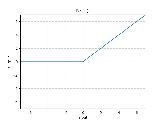
Let's look at some common activation functions. The graphs are from PyTorch's documentation.

Rectified Linear Unit (ReLu)

ReLu is generally most common activation function as it provides just enough nonlinearity to be useful, allows for quick learning, and is mathematically convenient. The output is:

\text{ReLu}(x) = \max(x, 0)

The graph follows directly as a regular linear line, cut off at $0$ for all negative values of $x$ .

Graph of ReLu Activation Function

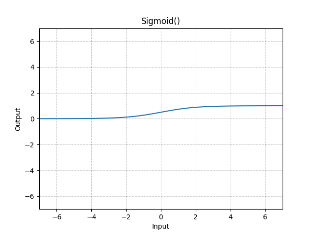
Sigmoid

The output of a sigmoid function is restricted between $0$ and $1$ , as you will see below, so it is usually used when you want to output a probability from the model (or any other value from 0 to 1).

\text{Sigmoid}(x) = \frac{1}{1 + e^{-x}}

The graph is:

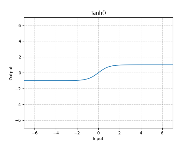
Graph of Sigmoid Activation Function

Tanh

The tanh activation function is analogous to the hyperbolic tangent function, meaning that the values are restricted between $-1$ and $1$ as shown:

\text{Tanh}(x) = \tanh{x} = \frac{e^x - e^{-x}}{e^x + e^{-x}}

Graph of Sigmoid Activation Function

We'll explore these activation functions (and their derivatives) more in the next section.

What Are Weights and Biases?

So far, we've talked about these arbitrary objects called weights and biases. Although they were defined vaguely, it's likely that what they are doesn't completely make sense yet. To define them, we need to discuss how the learning in neural networks happens.

Initially, these parameters are randomized by some algorithm. It turns out that the initial values of our weights and biases is very nontrivial. There are different methods of initialization that will be discussed later.

Learning in machine learning generally involves the tuning of some parameters such that the prediction gets closer and closer to the actual value. Likewise, neural networks learn by tuning internal parameters, called weights and biases, so that we get as accurate as possible. The actual process of how that is done is detailed in the next section.

There are also parameters that are generally not optimized within the model (they are still optimized, just in different ways). These are called hyperparameters. These are separate from the model parameters as the model parameters can be inferred directly from the data input. Some examples of hyperparameters in neural networks include the number of layers, the output dimensionalities of the layers, and the activation functions that are utilized.

Now that we have defined the structure of nonlinear and linear neural networks, we can put it all together into something called the forward pass. For each pass, we send in a batch of data $\mathbf{X}^{(i)}$ . There is one forward pass per batch, and a single epoch has $n$ forward passes, where $n$ is the number of batches. We will wrap up this whole process in the next section after we discuss backpropagation.

Going Backwards

Everything we've talked about so far---that is, the computation of the output of the neural network transformed by some weights and activation functions---is sometimes referred to as the forward pass (because we are going forward through each layer until we reach the output layer).

However, just giving us a prediction won't get us too far, because then our neural network would just be guessing. Let's explore how our neural network can learn the appropriate weights and biases for some data.

Measuring Inaccuracy

To learn anything, we also need to know what we are doing wrong. Neural networks learn from their mistakes, but this is only possible if we know how "much of a mistake" we are making. This means that we need some way to tell how innacurate our model is so that we can figure out what to do and when to stop.

A loss function quantifies this error, meaning that we have a scalar-valued function that returns a quantity representing the innacuracy of our model. There are various loss functions that are used in neural networks, but we will only be discussing the squared error loss function. It is defined as:

\text{MSE} = \frac{1}{n}\sum_{i = 1}^n(y_i-\hat{y}_i)^2

$n$ is the number of data points considered. The scalar output of this function gives a number that represents the overall innacuracy of the model.

Now, all that's left (and the fun part) is to minimize the innacuracy (therefore maximizing the accuracy) of the model.

Gradient Descent (GD)

We have a scalar valued function that returns the loss of the model given some weights and biases. If we can figure out the point at the global minimum of the loss function, we can find the weights that result in the lowest loss (resulting in the highest accuracy).

The idea is that we can use optimization methods to find this global minimum. Ideally, we would look for some type of analytical solution, but the functions outputted by neural networks generally don't allow for closed form solutions to finding the extremum.

For its computational efficiency and effectiveness, this optimization is done through an iterative process called gradient descent.

If you need a refresher on some of the concepts of calculus, look at the preliminaries section.

The Algorithm

We first start with some initial value of $\mathbf{W}_0$ . This represents the initial values of the weights we are updating in the network.

Assume that we already have the gradient of the weights with respect to the loss $\frac{\partial \mathcal{L}}{\partial \mathbf{W}}$ (we'll discuss how to compute this later). This shows us how the loss function changes in accordance with the weights.

Now, we set some arbitrary positive learning rates denoted $\{\eta_i\} > 0$ .

For $i = 1, 2, \dots$ (in the context of neural networks, we actually take one step for each forward pass of the network):

\mathbf{W}_{i + 1} = \mathbf{W}_i - \eta_i\nabla\mathcal{L}(\mathbf{W}_i)

Intuitively, we are taking a step in the opposite (negative) direction of the gradient for each iteration of the algorithm. Since the gradient points in the direction of the greatest increase, we are going to go in the opposite direction to travel towards the greatest decrease. If we keep going in this direction, we expect to eventually end up at a minimum.

The learning rate $\eta_i$ can also be thought of as the step size. One step in GD is defined as a single update of the weights. Varying this learning rate appropriately also leads to some interesting techniques that we will discuss.

It is important to note that in GD we expect to perform the forward pass for every single sample in the data set to perform a single update to the parameters. This will prove to be extremely inefficient for larger datasets.

Note that we update the biases in a similar fashion, taking $\frac{\partial \mathcal{L}}{\partial \mathbf{b}}$ instead of $\frac{\partial \mathcal{L}}{\partial \mathbf{W}}$ and adjusting the update rule appropriately.

There are other variants of gradient descent that are used in deep learning. Usually, libraries provide multiple "optimizers" (optimization algorithms) as certain algorithms perform better in certain scenarios. In this post, we'll only talk about one of those algorithms. Vanilla gradient descent (discussed in the previous section) is very uncommon for training neural networks.

Stochastic Gradient Descent (SGD)

Both gradient descent (GD) and stochastic gradient descent (SGD) are very similar. The difference in SGD is that we go forward for only a subset of data in the dataset instead of the entire dataset.

By doing this, we also get much noiser loss landscapes, meaning that we might be less likely to get stuck in a local minimum, as the noise sometimes causes the gradient to stray away from the local minima (and the global minimum).

Another technique, varying the learning rate, is often used to control the convergence of the algorithm. If we do not vary the learning rate, it can become very difficult to reach convergence at an optimal point.

It is especially important in SGD because of the noisiness of the objective function. In the gradient descent example, we had a set of constant learning rates for each iteration. However, decaying the learning rate exponentially (and other methods) also exist:

\eta(i) = \frac{\eta_0}{e^{\lambda i}}

In the exponential decay, $\lambda$ is known as the decay constant. It controls the rate at which the learning rate decays.

If we decay the learning rate too quickly, convergence time will increase significantly. However, if we don't decay enough, we risk not reaching the optimal point because of the all the noise.

In addition, sometimes the effectiveness of the learning rate differs for each dimension in the function. When the gradients are sufficiently low in one dimension but not so much in another, the effectiveness of the learning rate in one dimension might vary from another.

To compensate for this, we introduce the concept of momentum. Momentum allows us to fix this problem by taking into account the values of the previous gradients when taking the next step. More formally,

\mathbf{U}_{i + 1} = \alpha\mathbf{U}_i - \eta \nabla\mathcal{L}(\mathbf{U}_i)

\mathbf{W}_{i + 1} = \mathbf{W}_i + \mathbf{U}_i

With some substitution, we can rewrite this as a single update rule:

\mathbf{W}_{i + 1} = \mathbf{W}_i - \eta \nabla\mathcal{L}(\mathbf{U}_i) + \alpha\mathbf{U}_i

We also have a variable $0 \le \alpha \le 1$ that determines how "important" the previous gradient is for each step of gradient descent.

Overfitting and Regularization

In some cases, fitting our neural network to a dataset may result in something called overfitting. This happens when the neural network gets so "used to" the training data that the model won't give as accurate predictions when it encounters new, slightly different data.

The idea behind regularization is to solve this problem by putting a penalty on the weights in our loss function. Our previous loss function can be reiterated in terms of vectors $\mathbf{w}$ and $b$ as shown below:

\mathcal{L}(\mathbf{w}, b) = \frac 1 n\sum^n_{i = 1}(y^{(i)} - \hat{y}^{(i)})^2

With reguralization, we take the sum of this loss function and the norm of our weight vector, such that our loss becomes:

\mathcal{L}(\mathbf{w}, b) + \frac \lambda 2||\mathbf{w}||_n^2

Note that in $L_1$ regularization, $n = 1$ , and for $L_2$ regularization, $n = 1$ . Regularization is also called weight decay.

By doing this, we expect that if our weights get too big, our optimizer will eventually try to minimize the norm of the weights instead of just the loss. The parameter $\lambda > 0$ is what determines the magnitude of our penalty, and we can set $\lambda = 0$ to get our old loss function back. This is a hyperparameter (the meaning of this will be defined later) called the regularization constant. The multiplication by $\frac 1 2$ is simply for convenience, as the derivative settles nicely because the $2$ from the power cancels out with the division.

Assuming we are using SGD as our optimizer and $L_2$ regularization, we can also add the regularization to the update rule by taking its derivative:

\mathbf{w}_{i + 1} \leftarrow \mathbf{w}_i(1 - \eta_i\lambda) - \eta_i\nabla\mathcal{L}(\mathbf{w}, b)

Automatic Differentiation (Autodiff)

To compute the derivatives, namely $\frac{\partial \mathcal{L}}{\partial \mathbf{w}}$ and $\frac{\partial \mathcal{L}}{\partial \mathbf{\hat{y}}}$ , we use a method called automatic differentation. Automatic differentiation provides the numerical (not analytical) solution to the derivative of a function at a certain point.

There are two "variants" of automatic differentiation, each more efficient for a certain use case. For some function $f : \mathbb{R}^m \rightarrow \mathbb{R}^n$ , forward mode is more efficient when $m < n$ . In the other case, where $m > n$ , reverse mode is more efficient, and this it is what we use for computing derivatives in deep learning.

Overview

To understand the concept of reverse autodiff, we need to go back to the multivariable chain rule that we talked about in the beginning of this post.

For some function $\mathcal{L} : \mathbb{R}^n \rightarrow \mathbb{R}$ , we want the partial derivatives $\frac{\partial \mathcal{L}}{\partial x_1}, \dots, \frac{\partial \mathcal{L}}{\partial x_n}$ . To compute this in the human way, we would either take a limit or (preferably) use some of our handy rules of differentiation. Turns out that a computer isn't too different.

For some intuition before getting into the mathematics, we are going to split the computation of our gradient into two parts. First, we will go forward and record the operations that were done from our starting point in what is called a gradient tape. Then, we will go in backwards order and apply the derivative equivalent of the operation on the appropriate parameters, updating the gradients in accordance with the differentiation rules.

Say we have:

\mathcal{L}(x_1, x_2) = x_1x_2 + \sin(x_1) \text{ find } \frac{\partial \mathcal{L}}{\partial x} \text{ and } \frac{\partial \mathcal{L}}{\partial y}

We first rewrite this in terms of abstracted compositions of expressions:

\begin{align*} z & = \mathcal{L}(x, y) \\ & = \gamma_1\gamma_2 + \sin(\gamma_1) \\ & = \gamma_3 + \gamma_4 \\ & = \gamma_5\end{align*}

Now, we compute the value of $\gamma_5$ and record each of $\gamma_i$ in what is called the gradient "tape." Next, we go in the reverse order and compute the derivatives. However, let's first recall the chain rule for this context:

\text{For a function } f : \mathbb{R}^m \rightarrow \mathbb{R} \text{ in which } z = f \\\text{ and the argument of } f \text{ is a function } \mathbf{x}(t),

\frac{\partial z}{\partial t} = \sum_i \frac{\partial z}{\partial x_i}\frac{\partial x_i}{\partial t}

Using this rule, we can write $\frac{\partial z}{\partial \gamma_1}$ and $\frac{\partial z}{\partial \gamma_2}$ as a chained composition of $\gamma_3, \gamma_4, \gamma_5$ .

Now, let's go step by step for the reverse-mode differentiation:

\begin{align*}& \frac{\partial z}{\partial z} = 1 \text{ (seed)} \\& \frac{\partial z}{\partial \gamma_5} = 1 \\& \frac{\partial z}{\partial \gamma_4} = \frac{\partial z}{\partial \gamma_5} \frac{\partial \gamma_5}{\partial \gamma_4} = 1 \times 1 = 1 \\& \frac{\partial z}{\partial \gamma_3} = \frac{\partial z}{\partial \gamma_5} \frac{\partial \gamma_5}{\partial \gamma_3} = 1 \times 1 = 1 \\& \frac{\partial z}{\partial \gamma_2} = \frac{\partial z}{\partial \gamma_3} \frac{\partial \gamma_3}{\partial \gamma_2} + \frac{\partial z}{\partial \gamma_4} \frac{\partial \gamma_4}{\partial \gamma_2} = 1 \times \gamma_1 + 1 \times 0 = \gamma_1 \\ & \frac{\partial z}{\partial \gamma_1} = \frac{\partial z}{\partial \gamma_3} \frac{\partial \gamma_3}{\partial \gamma_1} + \frac{\partial z}{\partial \gamma_4} \frac{\partial \gamma_4}{\partial \gamma_1} = 1 \times \gamma_2 + 1 \times \cos(\gamma_1) = \gamma_2 + \cos(\gamma_1)\end{align*}

Notice how we went step by step in the backwards direction. If we program the basic derivative rules, we can see that adding a number $\gamma$ adds to the derivative of the parent operation to the current derivative, multiplying a number by another number $c$ adds the product of $c$ and the derivative of the parent operation, etc.

By generalizing these rules and chaining them together, we are able to compute the derivatives $\frac{\partial \mathcal{L}}{\partial x_1}, \dots, \frac{\partial \mathcal{L}}{\partial x_n}$ with complexity $\mathcal{O}(1)$ .

The final result from our computation above is:

\frac{\partial \mathcal{L}}{\partial x_1} = x_2 + \cos(x_1) \\ \frac{\partial \mathcal{L}}{\partial x_2}= x_1

In neural networks, the algorithm that computes the derivatives of the weight and bias objects is called backpropagation. Backpropagation uses reverse-mode automatic differentation to compute the gradients of the weights in the same way that is described above.

In case you need clarification, the functions produced by neural networks are not like the example function $\mathcal{L}$ shown above. They are made up of function composition (activation functions) and matrix multiplications (output of each layer).

Derivatives of Activation Functions

Generally, the derivatives of activation functions are hard-coded in deep learning libraries. Let's discuss these derivatives and their graphs here so that we can use them later in our implementations.

ReLu

$\sigma = \text{ReLu}(x)$

\frac{\partial \sigma}{\partial x} = \begin{cases}1 & \text{if }x > 0 \\ 0 & \text{if }x < 0 \end{cases}

Notice that the derivative is undefined at $x = 0$ . Generally it is rare to have $x$ at $0$ in the context of neural networks, so we just assume that the derivative is $1$ , $0$ , or $0.5$ for the sake of a cleaner and less error-prone implementation.

Sigmoid

$\sigma = \text{Sigmoid}(x)$

\frac{\partial \sigma}{\partial x} = \text{Sigmoid}(x)(1 - \text{Sigmoid}(x))

Tanh

$\sigma = \text{Tanh}(x)$

\frac{\partial \sigma}{\partial x} = 1 - \text{Tanh}^2(x)

The Backwards Pass

Now we have a set of tools for learning: a way to compute derivatives, some loss functions, and a number of methods for optimizing this loss function. Let's put this all together and create a concrete process that we can use to learn parameters in the network.

Let's say that at this point we have sent a batch of data $\mathbf{X}^{(i)}$ into the the network with some initial weights and biases. We now have an outputted prediction. This completes the forward pass for a single batch.

Now, we quantify the loss using a loss function, this is our objective function that will be minimized using our optimier. For this single batch, we take one step with our optimizer, and we are done with a full forward and backward pass of our neural network.

This process of forward pass, calculate loss, compute gradients, and update parameters is looped for every batch in our dataset and we take an optimizer step for every batch (every time we go forward). We repeat this process for $n$ number of epochs, where $1$ epoch is the completion of the forward and backward passes for every batch in the dataset.

This concludes the discussion of neural network theory. The next section deals with the technicalities that arise when we want to impelement neural networks in program code.

Computational Techniques

Let's take a step away from mathematics and towards engineering. The implementation of neural networks comes with some complexities and issues that need to be attended to in order to attain the most desirable results.

Model Parameters

Throughout the previous sections, we've talked about weights and biases. However, we only left these as arbitrary variables, because that is fine in mathematics. But, if we want to actually implement neural nets, it's important that we deal with real numbers, not variables.

When we say model parameters in the context of neural networks, we often mean the weights and biases of each layer. We already know from the previous section that the end values of our weights and biases will be the optimal weights and biases to minimize the loss for the given data. However, when starting out, how do we know what weights and biases to use?

We are more likely to get stuck in a local minimum if all of the weights are the same. In other words, all of the neurons will learn the same things and the network will be unable to generalize like we want it to.

In an attempt to optimize the initialization process, parameters are generally initialized using a recent method called kaiming initialization. We sample $W \sim \mathcal{N}(0, (\frac{2}{n_i})^{\frac 1 2})$ , where $n_i$ is the number of inputs to layer $i$ .

Tensors

Throughout the math for both the forward and backwards pass, we've talked about matrices and vectors. In the context of deep learning, these are simply convenient methods of representing data and computations involving them.

As you go deeper into your study of neural networks, you may find that we might need more than just a list, or a list of lists to store data. Thus, for mathematical convenience, we use tensors to represent data.

For context, a rank $2$ tensor can be represented as a matrix, and a rank $1$ tensor can be represented as a vector. Remember that the mathematical meaning behind these objects is not very useful to us, it's simply a more convenient and computationally efficient way to store information.

Moving forward in our implementations, we will use tensors to represent our data, weights, and biases.

From Theory To Implementation

Okay, so we now know how neural nets work mathematically and in theory. We also have some handy tricks for making neural networks easier to work with computationally. Now, it's time to actually make basic implementations of our theory. In this section, we'll be making a very basic neural network library.

One interesting exercise might be to follow along without referring to the code in the GitHub page. This will force you to write a large chunk of the automated differentiation API by yourself.

Note that implementing neural networks from scratch should, in most cases, never be done for practical use. There are existing libraries like PyTorch or Keras that allow for the same functionality and more in an efficient and stable manner.

Tensors

We'll make a very basic tensor class that stores a numpy ndarray as its elements. First, let's import numpy.

import numpy as np

Next, we can create our tensor class.

class Tensor:

The constructor simply stores the elements of the tensor as an ndarray and initializes the gradient objects (for autodiff).

For autodiff, we need to store a gradient "tape" that keeps track of all operations and also initialize our gradients to $0$ .

Note that we usually work with floating point numbers (float32) in deep learning. We only allow float Tensors for autodifferentiation.

def __init__(self, els, requires_grad=False, dtype=None, tape=None):    # Store the elements of our tensor in a numpy ndarray    self.els = np.array(els, dtype=dtype)    # Decide whether or not we are computing gradients    self.requires_grad = requires_grad    # Initialize an empty gradient tape for autodiff    self.tape = tape or []    # If the dtype is not "float", raise an error    if not self.els.dtype == float and requires_grad:        raise TypeError("Autodiff is only allowed for tensors of type \"float\"!")    # Otherwise, initialize our gradient    if requires_grad:        self.zero_grad()    else:       self.grad = None

Note that our zero_grad function is still not defined. The point of this function is exactly what it says---it initializes the gradient to an ndarray with zeros. The reason why we are making this a separate function is because we'll need it later for SGD.

def zero_grad(self):     self.grad = np.zeros_like(self.els)

We also need a way to make our Tensor subscriptable, meaning that if we try to get the $n$ th element of the tensor, we return the $n$ th item in the ndarray. For convenience, we'll also make sure that we return the els attribute of our Tensor object every time a user tries to print it.

def __getitem__(self, n):    return self.els[n]    def __repr__(self):    return self.els.__str__()

And we are now done with the base of our Tensor class.

Automated Differentiation

Next, let's implement autodiff. We will overload the multiplication, addition, subtraction, and division operations in the Tensor class.

Before we do that however, it's important to generalize all of our operations. Essentialy, we'll build an API for operations that have derivatives so that we can make our lives easier when actually implementing the operations. Our API takes in the following:

other - The other operand (other than self)

operation - A function that represents the operation that is to be performed

derivative_a - The function for the derivative of the first operand

derivative_b - The function for the derivative of the second operand

Using this, we can put together a function definition.

def __op(self, other, operation, derivative_a, derivative_b=None):

Note that we are not always guaranteed to have another Tensor as the other argument. An easy workaround to this would be to just convert it into one:

# Turn the other argument into a tensor if it isn't already oneif not isinstance(other, Tensor):    other = Tensor([other], dtype=self.els.dtype, requires_grad=False)

We also need to decide whether or not we want to compute gradients for this new output tensor. Generally, we want to if either one of our operands requires grad.

# If either one of our tensors require grad, then the output tensor also requires gradrequires_grad = self.requires_grad or other.requires_grad

Let's go ahead and compute the output. Note that we need to append the tapes of both this Tensor and the other Tensor to make sure that operations aren't left out when we chain them. If the gradient tape is out of order or has missing operations, our multivariable chain rule will not work.

Generally, this is taken care of by constructing a directed acyclic graph (DAG) and going backwards in topological order, but that is beyond the scope of our neural network library.

# Find the output tensor by executing the given operationout = Tensor(operation(self.els, other.els), requires_grad=requires_grad, tape=(other.tape + self.tape))

Finally, we add a function that computes the derivatives during the backwards pass. To prevent problems going forward, we'll also make sure to preserve the shapes of the outputs by summing the values on axis 0

def tape_action():   # Execute the derivative functions for the operation if the gradients exist  if self.grad is not None:     self.grad = self.grad + derivative_a(self.els, other.els, out.grad)    if self.grad.shape != self.els.shape:      self.grad = np.add.reduce(self.grad)  if other.grad is not None and derivative_b is not None:    other.grad = other.grad + derivative_b(self.els, other.els, out.grad)    if other.grad.shape != other.els.shape:      other.grad = np.add.reduce(other.grad)out.tape.append(tape_action)# Return the outputted valuereturn out

And the "API" is done.

Moving on to the actual operations, only a few are implemented here. For the full code, head over to the GitHub page.

Remember that our API takes in three functions:

operation(a, b) - The operation that is being performed, where a and b are the elements of the operands.

derivative_a(a, b, dc) - The derivative of a that is added to a.grad as per the chain rule. a and b are the elements of the operands and dc is the gradient of the output.

derivative_b(a, b, dc) - The derivative of b that is added to b.grad as described above.

Using this, let's override the __add__ method of our Tensor object:

def __add__(self, other):    return self.__op(other, lambda a, b: a + b, lambda a, b, dc: dc, lambda a, b, dc: dc)

Here, we have an anonymous function lambda a, b: a + b that reads, "the sum of a and b is a + b". The other two functions are a bit less obvious. Assuming that $z = c$ , and $c = a + b$ , we say that $\frac{\partial z}{\partial a} = \frac{\partial z}{\partial c}\frac{\partial c}{\partial a}$ , as per the chain rule. So we say that we add dc to the gradient of a for every addition operation.

The concepts are the same for subtraction, multiplication, etc.

def __sub__(self, other):    return self.__op(other, lambda a, b: a - b, lambda a, b, dc: dc, lambda a, b, dc: -dc)def __mul__(self, other):    return self.__op(other, lambda a, b: a * b, lambda a, b, dc: b * dc, lambda a, b, dc: a * dc)    # ... See the github page.

If you are interested in implementing autodiff by themselves, the list of operations that need to be supported are included below.

Addition

Subtraction

Multiplication

Division

Exponents

Summations (np.sum())

Negation

ReLU

Sigmoid

Tanh

Matrix Multiplication

Remember that the reverse operation functions, __rsub__, etc. must also be implemented.

Loss Functions

We now have completed most of what it takes to build neural networks. Implementing MSE is relatively straightforward. Recall that MSE is:

\text{MSE} = \frac{1}{n}\sum_{i = 1}^n(y_i-\hat{y}_i)^2

In our library, we will return a function that can be called to compute the loss, so that we can add additional options to the function (such as reduction, specifiying if we want to take the average or only the sum)

def MSE():   # Compute the mean squared error loss given a prediction (yhat) and a target (y)  def compute_loss(yhat, y):        N = np.prod(y.els.shape, dtype=float)    return ((y - yhat) ** 2).sum() / N  return compute_loss

That's it for loss functions!

Blocks (Modules)

Let's talk about how neural networks are structured. Anything that we can create should preferably be multipurposed for use for many different things.

In deep learning, we want to generalize the concept of a neural network to each of its components, such as activation functions, or layers. The easiest way to do this is to extract what all of these have in common: some inputs and some outputs. Even a single layer in a neural network is just an input-output gate. In fact, our entire neural network is an input-output gate.

To make use of this notion, we introduce the concept of blocks, or modules. A module is simply an object that holds some parameters, takes in an input, and transforms it to create an output. Modules can be put together to form layers, groups of layers, or neural networks.

Let's implement this, starting off with a base class.

class Module:   def __init__(self, *args):     # Initialize module with given arguments as children    self.__children = args or []           def forward(self, x):    # Call .forward() on all of the children    for child in self.__children:      x = child.forward(x)    return x

We also need a way to keep track of block parameters. To identify parameters, we can create a very basic class:

class Parameter:   def __init__(self, data, requires_grad=True):    # Set data of parameter    self.data = Tensor(data, requires_grad, float)

This will just be a convenient way to keep track of module parameters. It also helps to have a convenient way to get all of the parameters in a module:

# Note: This is a method in the module classdef parameters(self):    # Fetch all of the parameters by going through each child    parameters = []    for child in self.__children:      for (key, value) in child.__dict__.items():        if isinstance(value, Parameter):          parameters.append(value)    return parameters

And that's it, we've successfully implemented modules.

Layers

Using our modules, it helps to give users some starter layers so that they can build their own neural networks.

Starting off with the linear module, we initialize the weights and biases with kaiming initialization. We then override the forward function with the output computation of a linear layer, $\mathbf{X}\mathbf{W} + \mathbf{b}$ .

# Just a basic linear layer with an optional bias nodeclass Linear(Module):  def __init__(self, input_neurons, output_neurons, bias=True):    self.weights = Parameter(np.random.normal(0,                                              (2 / input_neurons)**1/2,                                              (input_neurons, output_neurons)))    self.bias = bias    if bias:      self.biases = Parameter(np.random.randn(output_neurons))  def forward(self, x):    out = x.matmul(self.weights.data)    if self.bias:       return out + self.biases.data    return out

We can add activation functions using the same concept:

class ReLU(Module):  def forward(self, x):    return x.relu()class Sigmoid(Module):  def forward(self, x):    return x.sigmoid()class Tanh(Module):  def forward(self, x):    return x.tanh()

Stochastic Gradient Descent

We've reached the final part of our library: optimization.

Our optimizer will be a class, one with a function called step(). The purpose of this function is to to take a single gradient step for every parameter in the network. This is usually called for every time we go forward with a batch of data. Every class instance will store the parameters that we are trying to optimize.

First we can set up a base class, taking in the parameters we want to optimize and the learning rate of the algorithm:

class SGD:   def __init__(self, parameters, learning_rate):    self.parameters = parameters    self.learning_rate = learning_rate

Next, we implement SGD as shown here. We also can pass an argument that resets the gradients so that we have an accurate computation for the next forward pass.

def step(self, zero_grad=False):    for param in self.parameters:       param = param.data # Get the data inside the parameter      # w_i+1 <- w_i - lr * (dL/dw_i)      param.els = param.els - self.learning_rate * param.grad      # Reset the gradient if specified      if zero_grad:        param.zero_grad()

To end it off, we can add another zero_grad method for convenience and flexibility:

def zero_grad(self):     for param in self.parameters:       param.zero_grad()

We've now built a basic neural network library! To see the code in more detail, see the github page. If you've made it this far, thanks for reading. I hope you've learned something out of this. For a more in-depth and complete resource for implementing and understanding neural networks, try the free ebook Dive into Deep Learning

Last Updated: December 2021